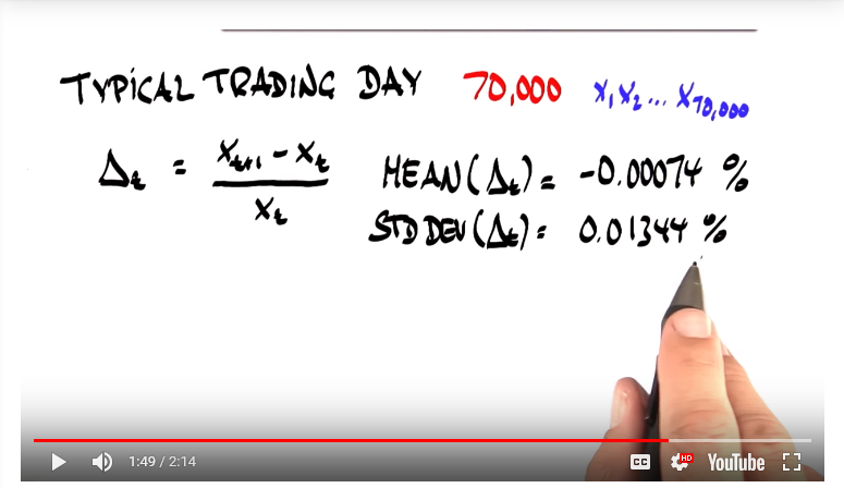
33. Flash Crash Example
import numpy as np # linear algebra
import pandas as pd # data processing, CSV file I/O (e.g. pd.read_csv)
btc=pd.read_csv("../input/bitstampUSD_1-min_data_2012-01-01_to_2018-11-11.csv")  #importing csv file
btc.head()
Cleanup the data
btc = btc.dropna()  # remove NaN they do not help
btc["Timestamp"]=pd.to_datetime(btc["Timestamp"],unit="s")

hour=btc["Timestamp"]==btc["Timestamp"].dt.floor("H")  # there are over 3 million entries in the dataframe
df=btc[hour]                                    # to make the dataset more simple i only take daily values

df = df[(df['Timestamp'] > '2017-06-20 00:00:00') & (df['Timestamp'] <= '2017-07-23 00:00:00')]
df.head()
Calculate $\Delta$T
Each $\Delta_t$ at"t"th moment can be defined as b
$$ \Delta_t = \dfrac{X_{t+1} - X_t }{X_t} $$
df['dX'] = (df['Weighted_Price'].shift(-1) - df['Weighted_Price'])/df['Weighted_Price'].shift(-1)
df['dX'] = df['dX'].shift(1)
# df['dX'] = df['dX'].round(5)  # rounding to 3 decimal places for better frequency distribution later
df = df.dropna()
df.head()
Plot
import matplotlib.pyplot as plt
fig,axr = plt.subplots(2,1,figsize=(14,5))

T = df.Timestamp
X = df.Weighted_Price
dX = df.dX

ax = axr[0]
ax.plot(T,X , color="green", label="BTC/USD")      # line plot for seeing the daily weighted price
ax.set_xlabel ("Time")
ax.set_ylabel("USD")

ax = axr[1]
ax.plot(T,dX , color="green", label="BTC/USD")      # line plot for seeing the delta
ax.set_xlabel ("Time")
ax.set_ylabel("USD_Normalized_Delta")

plt.legend()
plt.show()
Sampling Distribution of Delta X
Let us analyze that, how it looks like to get an idea. Note, this frequency is for a particular time window. If window changes, these could change.
# freq = df['dX'].value_counts()
X = df['dX'].tolist()

fig, ax = plt.subplots(1,1, figsize=(7,5))

ax.hist(X, bins=50)

from matplotlib.ticker import FormatStrFormatter
ax.xaxis.set_major_formatter(FormatStrFormatter('%.4f'))
plt.show()
Strange. The delta differences follow a normal distribution. With the mean almost zero. Let us calculate the $\overline{x}$ and $s$ precisely.
mean = sum(X)/len(X)
var = sum([ (i - mean)**2 for i in X ])/len(X)
from math import sqrt
sd = sqrt(var)
meanstr = str.format('{0:.6f}', mean) # this is a string to print in desired decimal places
sdstr = str.format('{0:.6f}', sd)
print(meanstr, sdstr)
Note, the values we got are similar (not equal though ofcourse) to what Sebastian writes (Psst! that is in percentage)
Thus, we are not only convinced of the values, but also that, we see, the normalized delta forming a normal distribution, we are convinced of taking confidence intervals which should hold good because the given distribution is already normal. Let us take CI for our own values, like how Sebastian does and observe the outcome.
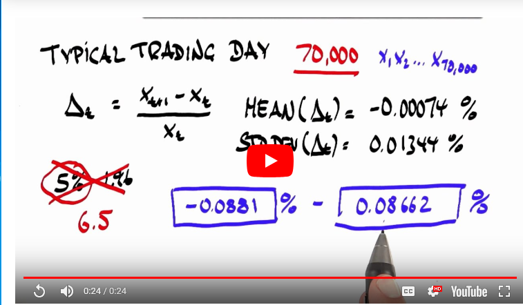
$$ \overline{x} = 0.000042 \ \ \ \ s = 0.009951 \ \ \ \ n = 1 \\ CI = \overline{x} \pm 1.96\dfrac{s}{\sqrt{n}} = ? $$
n = 1 # because each sample set size is 1
l_ci, h_ci = mean - 1.96*(sd/sqrt(n)), mean + 1.96*(sd/sqrt(n))
round(l_ci,4), round(h_ci,4)
Quiz: Outlier Frequency
For how many cases will we expect out measurement to fall outside the interval?
from IPython.display import HTML
html = '<iframe width="418" height="235" src="https://www.youtube.com/embed/xku0dnLWkcI" frameborder="0" allow="accelerometer; autoplay; encrypted-media; gyroscope; picture-in-picture" allowfullscreen></iframe>'
HTML(html)
This depends on our window. Our total sample sets could be counted, and as per confidence interval, about 5% of them are expected to fall outside the range.
total_samples = len(X)
n_outliers = total_samples*0.05  # about 5% are expected to fall outside as per the distribution we saw earlier
print(total_samples, n_outliers, (n_outliers/total_samples)*100)
Thus out of 787 samples, we could expect about 40 samples to fall outside the range of CI in our given window.
New Interval
Now Sebastian takes the game to a new (significance) level. This time, instead of z = 1.96, we take z = 6.5, as you can see in normal distribution this is really a rare case.
$$ \overline{x} = 0.000042 \ \ \ \ s = 0.009951 \ \ \ \ n = 1 \\ CI = \overline{x} \pm 6.5\dfrac{s}{\sqrt{n}} = ? $$
n = 1 # because each sample set size is 1
l_ci, h_ci = mean - 6.5*(sd/sqrt(n)), mean + 6.5*(sd/sqrt(n))
round(l_ci,4), round(h_ci,4)
This is also similar to values Sebastian got
Basic Indicator
Now that we have the lower and upper limits, let us try constructing a simple indicator. If the delta is out of the lower range of CI, we will raise an alarm (to sell). Since our chosen window is not having a dramatic crash as Sebastian used, we shall use our previous outliers of 5% (that is 1.96).
df['dI'] = 0
# df.loc[df['dX'] > 0.0195, 'dI'] = 1   # using 5% significance as we do not have much of crash in our chosen window
df.loc[df['dX'] < -0.0195, 'dI'] = 1
df.head()
fig,axr = plt.subplots(3,1,figsize=(14,5))

T = df.Timestamp
X = df.Weighted_Price
dX = df.dX
dI = df.dI

ax = axr[0]
ax.plot(T,X , color="green", label="BTC/USD")      # line plot for seeing the daily weighted price
ax.set_xlabel ("Time")
ax.set_ylabel("USD")

ax = axr[1]
ax.plot(T,dX , color="green", label="BTC/USD")      # line plot for seeing the delta
ax.set_xlabel ("Time")
ax.set_ylabel("USD_Normalized_Delta")

ax = axr[2]
ax.plot(T,dI , color="green", label="BTC/USD")      # line plot for seeing the delta
ax.set_xlabel ("Time")
ax.set_ylabel("Indicator")

plt.legend()
plt.show()
Depending on the crash level, one could choose the confidence level, and thus wider range. For eg, 1.96 gives many alarms as above, which may be useful to some, but others may prefer a wider interval to only indicate a bigger crash. They could simply choose a higher confidence level.